Announcement
Comparing Two Measurement
Devices
Part I
It's rare when a paper says everything that needs to be said in a way
that can be readily understood by a nontechnical audience, but this is
one of those cases. The paper is "Statistical Methods for Assessing
Agreement Between Two Methods of Clinical Measurement," by JM Bland and
DG Altman (The Lancet, February 8, 1986, 307-310). Perhaps it is so
approachable because it was written for medical researchers three years
after an equally readable version appeared in the applied statistics
literature (Altman and Bland, 1983) and about the same time as a heated
exchange over another approach to the problem (Kelly, 1985; Altman and
Bland, 1987; Kelly, 1987).
This could very well have been a two-sentence note: "Here's the Bland
and Altman reference. Please, read it." Still, its message is so elegant
by virtue of its simplicity that it's worth the time and space to review
the approach and see why it works while other approaches do little more
than confuse the issues.
The Problem
Suppose there are two measurement techniques*, both of
which have a certain amount of measurement error**, and we
widh to know whether they are comparable. (Altman and Bland use the
phrasing, "Do the two methods of measurement agree sufficiently
closely?") Data are obtained by collecting samples and splitting them in
half. One piece is analyzed by each method.
The meaning of "comparable" will vary according to the particular
application. For the clinician, it might mean that diagnoses and
prescriptions would not change according to the particular technique that
generated a particular value. For the researcher, "comparable" might mean
being indifferent to (and not even caring to know) the technique used to
make a particular measurement--in the extreme case, even if the choice
was made purposefully, such as having all of the pre-intervention
measurements made using one technique and the post-intervention
measurements made with the other. (This would always make me
nervous, regardless of what had been learned about the comparability of
the methods!)
The Bland-Altman approach is so simple because, unlike other methods,
it never loses focus of the basic question of whether the two methods of
measurement agree sufficiently closely. The quantities that best answer
this question are the differences in each split-sample, Bland and Altman
focus on the differences exclusively. Other approaches, involving
correlation and regression, can never be completely successful because
they summarize the data through things other than the differences.
The Bland-Altman papers begin by discussing inappropriate methods and
then shows how the comparison can be made properly. This note takes the
opposite approach. It first shows the proper analysis and then discuss
how other methods fall short. In fact, this note has already presented
the Bland-Altman approach in the previous paragraph--do whatever you can
to understand the observed differences between the paired measurements:
- Plot the two sets of measurements along with the line
Y=X. If the measurements are comparable, they will be tightly
scattered about the line.
- Because the eye is better at judging departures from
a horizontal line than from a tilted line, plot the difference
between a pair of measurements against their mean. If the
measurements are comparable, the differences should be small,
centered around 0, and show no systematic variation with the
mean of the measurement pairs. Those who like to supplement
plots with formal analysis might a construct confidence
interval for the mean difference and test the statistical
significance of the correlation coefficient between the sums
and differences.
- Assuming no warning signs are raised by the plot in
part (2), (that is, if the observations are centered around 0
and there is no systematic variation of the difference with
the mean) the data are best summarized by the standard
deviation of the differences. If this number is sufficiently
small from a practical (clinical) standpoint, the measurements
are comparable.
Examples
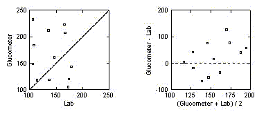 These data represent an
attempt to determine whether glucose levels of mice determined by a
simple device such as a Glucometer could be used in place of standard lab
techniques. The plots of Glucometer value against lab values and their
difference against their mean shows that there is essentially no
agreement between the two measurements. Any formal statistical analyses
would be icing for a nonexistent cake!
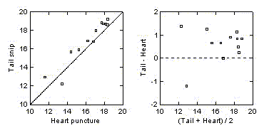 These data represent an
attempt to determine whether vitamin C levels obtained from micro-samples
of blood from tail snips could be used in place of the standard technique
(heart puncture, which sacrifices the animal). The plots clearly
demonstrate that the tail snips tend to give values that are 0.60 units
higher than the standard technique. With a standard deviation of the
differences of 0.69 units, perhaps the tail snip could be of practical
use provided a small downward adjustment was applied to the measurements.
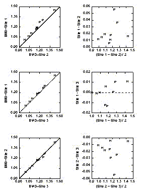 These data come from a study
of the comparability of three devices for measuring bone density. The
observations labelled 'H' are human subjects; those labelled 'P' are
measurements made on phantoms. Since there are three devices, there are
three pairs of plots: 1/2, 1/3, 2/3. Here we see why the plot of one
measurement against another may be inadequate. All three plots look
satisfactory. However, when we plot the differences against the mean
values, we see that the measurements from site 2 are consistently less
than the measurements from the other two sites, which are comparable.
Comment
It may take large samples to determine that there is no statistically
significant difference of practical importance, but it often takes only a
small sample to show that the two techniques are dramatically different.
When it comes to comparability, the standard deviation of the differences
is as important as their mean. Even a small sample can demonstrate a
large standard deviation.
Other Approaches and Why They Are Deficient
- Paired t tests test only whether the mean responses are
the same. Certainly, we want the means to be the same, but this is only a
small part of the story. The means can be equal while the (random)
differences between measurements can be huge.
- The correlation coefficient measures linear
agreement--whether the measurements go up-and-down together. Certainly,
we want the measures to go up-and-down together, but the correlation
coefficient itself is deficient in at least three ways as a measure of
agreement.
- The correlation coefficient can be close to 1 (or equal to 1!)
even when there is considerable bias between the two methods. For
example, if one method gives measurements that are always 10 units higher
than the other method, the correlation will be 1 exactly, but the
measurements will always be 10 units apart.
- The magnitude of the correlation coefficient is affected by the
range of subjects/units studied. The correlation coefficient can be made
smaller by measuring samples that are similar to each other and larger by
measuring samples that are very different from each other. The magnitude
of the correlation says nothing about the magnitude of the differences
between the paired measurements which, when you get right down to it, is
all that really matters.
- The usual significance test involving a correlation coefficient--
whether the population value is 0--is irrelevant to the comparability
problem. What is important is not merely that the correlation coefficient
be different from 0. Rather, it should be close to (ideally, equal to) 1!
- The intra-class correlation coefficient has a name
guaranteed to cause the eyes to glaze over and shut the mouth of anyone
who isn't an analyst. The ICC, which takes on values between 0 and 1, is
based on analysis of variance techniques. It is close to 1 when the
differences between paired measurements is very small compared to the
differences between subjects. Of these three procedures--t test,
correlation coefficient, intra-class correlation coefficient--the ICC is
best because it can be large only if there is no bias and the
paired measurements are in good agreement, but it suffers from the same
faults ii and iii as ordinary correlation coefficients. The magnitude of
the ICC can be manipulated by the choice of samples to split and says
nothing about the magnitude of the paired differences.
- Regression analysis is typically misused by regressing one
measurement on the other and declare them equivalent if and only if the
confidence interval for the regression coefficient includes 1. Some
simple mathematics shows that if the measurements are comparable, the
population value of the regression coefficient will be equal to the
correlation coefficient between the two methods. The population
correlation coefficient may be close to 1, but is never 1 in practice.
Thus, the only things that can be indicated by the presence of 1 in the
confidence interval for the regression coefficient is (1) that the
measurements are comparable but there weren't enough observations to
distinguish between 1 and the population regression coefficient, or (2)
the population regression coefficient is 1 and therefore, the
measurements aren't comparable.
- There is a line whose slope will be 1 if the measurements are
comparable. It is known as a structural equation and is the method
advanced by Kelly (1985). Altman and Bland (1987) criticize it for a
reason that should come as no surprise: Knowing the data are consistent
with a structural equation with a slope of 1 says something about the
absence of bias but *nothing* about the variability about Y = X (the
difference between the measurements), which, as has already been stated,
is all that really matters.
The Calibration Problem
Calibration and comparability differ in one important respect. In the
comparability problem, both methods have about the same amount of error
(reproducibility). Neither method is inherently more accurate than the
other. In the calibration problem, an inexpensive, convenient, less
precise measurement technique (labelled C, for "crude") is compared to an
expensive, inconvenient, highly precise technique (labelled P, for
"precise"). Considerations of cost and convenience make the crude
technique attractive despite the decrease in precision.
The goal of the calibration problem is use the value from the crude
method to estimate the value that would have been obtained from the
precise method. This sounds like a problem regression in regression,
which it is but with a twist!
With ordinary regression, an outcome variable (labelled Y) is
regressed on an input (labelled X) to get an equation of the form Y = a +
b X. However, the regression model says the response for fixed X varies
about the regression line with a small amount of random error. In the
calibration problem, the error is attached to the predictor C, while
there is no error attached to P. For this reason, many authors recommend
the use of inverse regression, in which the crude technique is regressed
on the precise technique (in keeping with the standard regression model:
response is a linear function of the predictor, plus error) and the
equation is inverted in order to make predictions. That is, the equation
C = b0 + b1 P is obtained by least squares
regression and inverted to obtain
P = (C - b0) / b1
for prediction purposes. For further discussion, see Neter,
Wasserman, and Kutner (1989, sec 5.6).
The calibration literature can become quite confusing (see Chow and
Shao, 1990, for example) because the approach using inverse regression is
called the "classical method" while the method of regressing P on C
directly is called the "inverse method"!
--------------------------
*Device would be a better work than
technique. I've seen the Bland-Altman method used in situations
where one or both of the "techniques" were prediction equations. This
might be appropriate according to the error structure of the data, but it
is unlikely that such an error structure can be justified.
**Even gold standards have measurement error. The
Bland-Altman technique assumes the measurement errors of the two devices
are comparable. This will be discussed further in Part II.
References
- Altman DG and Bland JM (1983), "Measurement in Medicine: the Analysis
of Method Comparison Studies, " The Statistician, 32, 307-317.
- Altman DG and Bland JM (1987), Letter to the Editor. Applied
Statistics, 36, 224-225.
- Chow SC and Shao J (1990), "On the Difference Between the Classical
and Inverse Methods of Calibration," Applied Statistics, 39, 219-228.
- Kelly GE (1985), "Use of the Structural Equation Model in Assessing
the Reliability of a New Measurement Technique," Applied Statistics, 34,
258-263.
- Kelly GE (1987), Letter to the editor. Applied Statistics, 36, 225-
227.
- Neter J, Wasserman W, and Kutner M (1989), Applied Linear Regression
Models. Boston, MA: Richard D. Irwin.
Copyright © 2000 Gerard E. Dallal
 These data represent an
attempt to determine whether glucose levels of mice determined by a
simple device such as a Glucometer could be used in place of standard lab
techniques. The plots of Glucometer value against lab values and their
difference against their mean shows that there is essentially no
agreement between the two measurements. Any formal statistical analyses
would be icing for a nonexistent cake!
  These data represent an
attempt to determine whether vitamin C levels obtained from micro-samples
of blood from tail snips could be used in place of the standard technique
(heart puncture, which sacrifices the animal). The plots clearly
demonstrate that the tail snips tend to give values that are 0.60 units
higher than the standard technique. With a standard deviation of the
differences of 0.69 units, perhaps the tail snip could be of practical
use provided a small downward adjustment was applied to the measurements.
 These data come from a study
of the comparability of three devices for measuring bone density. The
observations labelled 'H' are human subjects; those labelled 'P' are
measurements made on phantoms. Since there are three devices, there are
three pairs of plots: 1/2, 1/3, 2/3. Here we see why the plot of one
measurement against another may be inadequate. All three plots look
satisfactory. However, when we plot the differences against the mean
values, we see that the measurements from site 2 are consistently less
than the measurements from the other two sites, which are comparable.